
Screening Model
On the test-run of Version 1.0 of Tuberculosis Classification Model, a need for segregating good quality Chest X-Rays from X-rays of other body parts was realized.
Accordingly I tried out two approaches:
1) Anomaly detection techniques
2) Classification
1) Anomaly detection Techniques:
Historically One Class Svm is a hit and miss in scenarios where only one class/type of data is known and the other class can be virtually anything. Since I had no image data on what other kind of X-rays I could encounter, I tried one-class SVM with gaussian mixture models.
In the meanwhile I worked on extracting the images belonging to the “Other” class from DMH data so as to apply a straightforward Bi-classification.
I trained the One-Class on Chest X-Rays from NIH and extracted features using Alexnet architecture. I reduced the features to about a 1000 per image, by directly taking the probabilities assigned to each class from the last layer Fully connected FC layer. Previous attempts for taking 4096 features and applying transfer learning with vanilla One Class Svm from sklearn yielded poor results.
In one class Svm I tried approach I further tried out three approaches, details are given below
Datasets : Train : 2000 Chest-x-rays
Test: 450 Chest-x-rays
412 Various X-rays
- a) One class SVM : accuracy 72.73%
- b) Isotation Forests : accuracy 87.00%
- c) Gaussian Mixture with isotonic regression : accuracy 95.12%
The 412 X-rays labels various X-rays were taken from Openly available dataset on Kaggle, from sources MRI dataset and RSA Bone age
Below are the results of the Gaussian Mixture Model:
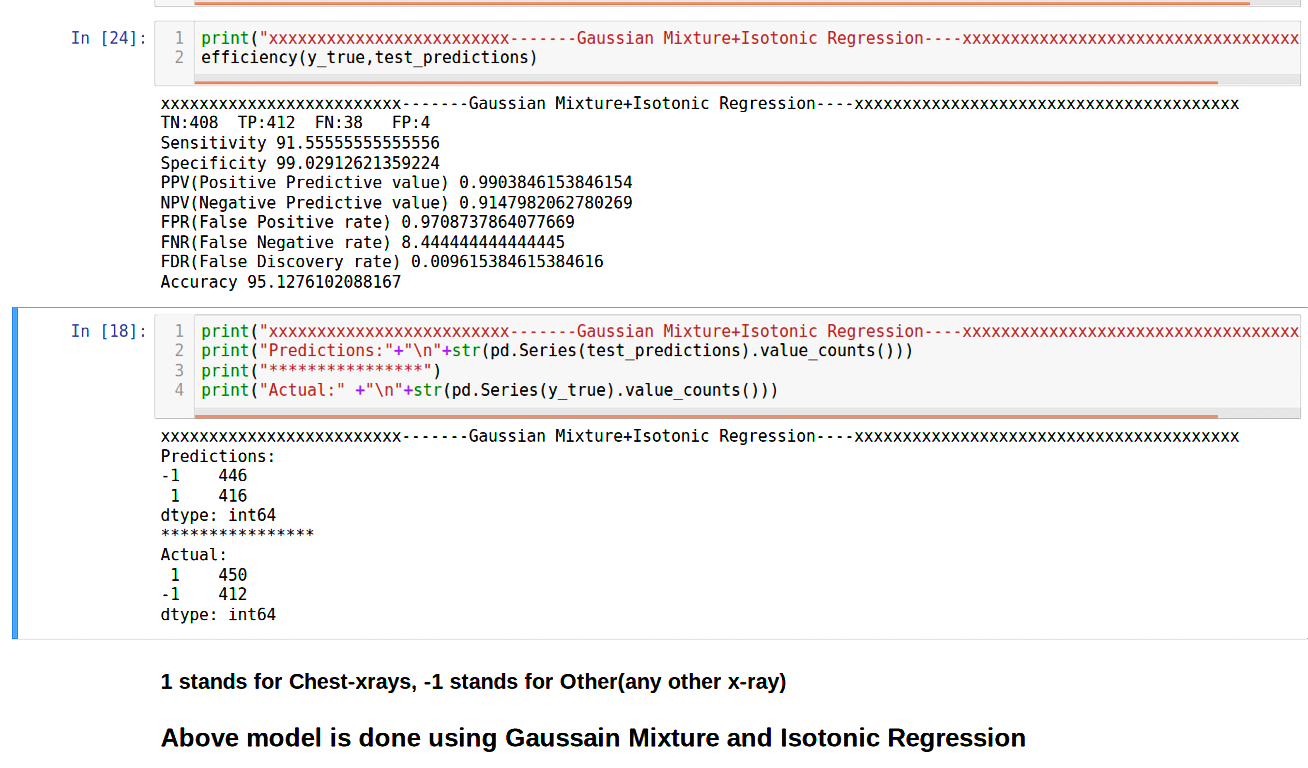 In the above experiments I chose a threshold of 0.5. If the predict probability is above 0.5 only then the image is classified as a Chest X-Ray. To make sure that the ones predicted as Chest X-Rays are indeed their namesake(reducing False Positives or FP) I increase the threshold. Naturally the Positive Predictive Rate increases. Look at the formula to ascertain.
You might be wondering that doing so would increase False Negatives(Actually Positive but termed as Negative).In some cases it is fatal, imagine if I were predicting chance of Cancer and our model had high number of cases of Cancer being labelled as Non-Cancer.
However, in our model I want to increase Specificity(measures the rate of truly identifying the Other X-Rays), it is okay if I do so at the cost of losing out on Sensitivity(measures the proportion of positives that are correctly identified as such).
In all other scenarios a trade off between the above two is established with the F1 score and an apt threshold is selected
a) One Class SVM with radial kernel
One-class SVM is used for novelty detection, that is, given a set of samples, it will detect the soft boundary of that set so as to classify new points as belonging to that set or not. In this case, as it is a type of unsupervised learning, the model is fit only on data from the positive class, there is no negative class
b) Isolation Forests
The Isolation Forest ‘isolates’ observations by randomly selecting a feature and then randomly selecting a split value between the maximum and minimum values of the selected feature. Since recursive partitioning can be represented by a tree structure, the number of splittings required to isolate a sample is equivalent to the path length from the root node to the terminating node. This path length, averaged over a forest of such random trees, is the anomaly score. This anomaly score(path lengths) is used to tell apart outliers from normal observations. Random partitioning(feature selection to partition data,selects best feature in every iteration) produces noticeably shorter paths for anomalies. Hence, when a forest of random trees collectively produce shorter path lengths for particular samples, they are highly likely to be anomalies. A visual approach on the inner workings is provided here.
c) Gaussian Mixture Models
They are a probabilistic model for representing normally distributed subpopulations within an overall population”. It can be surmised that a mixture model represents clusters of normally distributed subpopulations. A Gaussian mixture model, once fitted on the data, can give us information on the probability of whether any new point was generated from that distribution.
Gaussian mixture models return log of probability density function values for a given sample (and not actual probabilities). Hence it is necessary to convert these probability density function values to ‘probability scores’, which can then show that a new sample will belong to the Gaussian distribution with “x” amount of confidence. I accomplished this by fitting an isotonic regression model on the log probability density scores w.r.t. labels for the validation set data points. Isotonic regression is a probability calibration technique which can calibrate classifier scores to approximate probability values by fitting a stepwise non-decreasing function along the scores returned by the classifier. Read this fascinating insight on Why do we need Calibration? for details.
I validated this Gaussian Mixture Model on DMH dataset(data provided from a hospital) and it performed poorly, only recognizing ~50% of the images. I suspected this had something to do with overfitting to data source.
2) Classification
Since the results of Anomaly detection were poor. I tried out a Classification approach to segregate good quality Chest X-Rays from X-rays of other body parts. For this to work I needed good training data which was provided by a local hospital. I shall refer to this data as DMH dataset henceforth. DMH stands for Deenanath Mangeshkar Hospital
a) Bi-classification
I segregated Chest X-Rays from other X-Rays from DMH dataset. Various X-rays included X-Rays from Knee, Hands, Mammograms and Pediatrics, of varying distributions
Datasets : Train : 1000 Chest-X-rays
1000 Various X-rays
Test: 500 Chest-X-rays
500 Various X-rays
I used the same model used for Tuberculosis Classification , a Chexnet based approach for extracting features. There were 1024 features per image, I applied average Pool, cuz our model gave 50176 features. To apply decision trees with this number of features would cause overfitting due to high dimentionality.Tips on practical use
So to reduce features instead of applying a PCA or Feature Selection before giving them to decision trees for classification , I apply a nueral-net natural approach i.e Pooling. There are two kinds of Pooling, Average and Max. Max pooling is better suited for retaining extreme features such as edges,whereas Average pooling helps with a more smoother transition I have used Global average pooling here is a pictorial representation of what it does:

So I now reduced the 50176 features per image to just 1024 features. I have 2000 Training images so number of features < < number of images(1024<2000) We can be confident that the model wont overfit now, atleast due to excess features. With transfer learning and features extracted I then applied Random Forests, to classify between Chest X-Rays and Other X-Rays.
Following are the Results from the 10-fold cross validation:
| Metric | Score |
|---|---|
| Sensitivity | 94.8 |
| Specificity | 98.2 |
| PPV(Positive Predictive value) | 0.98 |
| NPV(Negative Predictive value) | 0.95 |
| FPR(False Positive rate) | 1.80 |
| FNR(False Negative rate) | 5.20 |
| FDR(False Discovery rate) | 0.018 |
| Accuracy | 0.96 |
To increase Specificity and PPV, for reasons stated previously I performed a threshold comparison and chose a threshld of 0.8
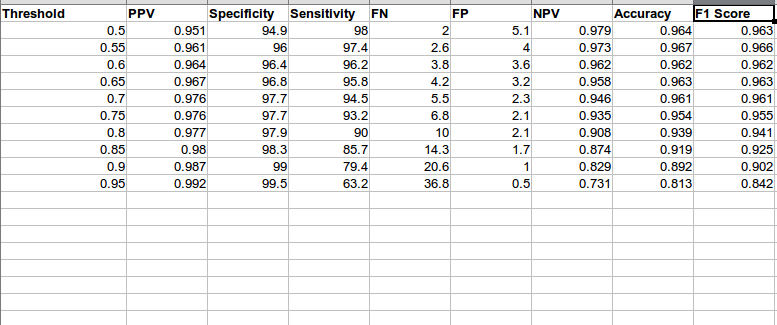
As you can see as threshold increases FP(False Positive) reduce and FN(False negative) increase
I then tested the data, on the Test data mentioned above, following were the results:
| Metric | Score |
|---|---|
| Sensitivity | 91.06 |
| Specificity | 98.4 |
| PPV(Positive Predictive value) | 0.98 |
| NPV(Negative Predictive value) | 0.92 |
| FPR(False Positive rate) | 1.60 |
| FNR(False Negative rate) | 8.40 |
| FDR(False Discovery rate) | 0.017 |
| Accuracy | 0.95 |
The Results, were promising and I integrated the Screening model in our application You can view a demo here. Besides, the above results the model could screen the data from RSNA bone images and MRI Images. I never used them for training or testing, this was truly novel data. The model was also able to screen blurry images with a prompt on whether the User would like to proceed to predicting Tuberculosis on the X-ray Image anyway.