
More than 250 years ago, the challenge of making predictions from small data weighed strongly on presbyterian minister Reverend Bayes of Tunbridge Wells, England.
Looking to the easily banal Raffles of the 18th Century England he wondered what one’s chances of winning them were. If five tickets out of ten bought won, then the chances of a win were quite simply 50%. But what if one bought a single ticket and it came out the winner? Were the chances of winning the Raffle really a 100%? It sounded far too simplistic to our dear Reverend who balanced scholarly and theological interests almost all his life. Ordained like his father and a man of keen intellect he was elected to the Royal Society in 1742.1
For somebody who had such an immense impact in the field of reasoning under uncertainty, little can be said about Bayes’s history with certainty. He is certainly known to have published two works in his lifetime, one theological and one mathematical:
- Divine Benevolence, or an Attempt to Prove That the Principal End of the Divine Providence and Government is the Happiness of His Creatures (1731)
- An Introduction to the Doctrine of Fluxions, and a Defence of the Mathematicians Against the Objections of the Author of The Analyst (published anonymously in 1736), in which he defended the logical foundation of Isaac Newton’s calculus (“fluxions”) against the criticism of George Berkeley, author of The Analyst
However, we have no records of his other published works. Be that as it may, we know for certain that his work and findings on probability theory were passed in manuscript form to his friend Richard Price after his death. For it was in his friend’s perusal that Bayes’s Critical Insight underlying the elegance of the Bayes theorem came into light.
Bayes noted that ‘Reasoning forward from hypothetical pasts lays the foundation for us to then work backward to the most probable past.’ He explained that if we bought three tickets and all three of them are winners then the chances of winning were 100%, a rather generous find. If half of the tickets sold in a raffle are winners then our chances are i.e . If the raffle awarded only 1 in thousand tickets then our chances of winning in the three tickets bought are i.e Bayes ‘s logic quantifies our intuition that it is exactly 8 times likelier that all tickets are winners than half of them are. Furthermore it is exactly 125 million times likelier that half of them are winners as opposed to 1 in a thousand. He probably came up with this Critical Insight in an experiment where he sat with his back to a perfectly round, perfectly square table and asked his assistant to throw a ball on the table and describe its position, using the words “left”, “right” “front” and “back”. He noted it down on his pad and consistently made his hypothesis about the original position of the ball better. But the insight never saw ink to paper as Bayes probably abandoned the same, thinking of it as rather ordinary, common knowledge.
Thinking back to our example, what are the odds of winning a raffle away? In 1774, Laplace solved the problem of making inferences backwards from their observed effects to their probable causes.Laplace was born in Normandy in 1749, and his father sent him to the University of Caen to study theology.Unlike, Bayes Laplace abandoned his theist persuit entirely for mathematics. Using Calculus, Laplace could distill the vast number of hypotheses( as in the case of a raffle) to a single concise value with a superbly succinct formula where w is number of winning tickets in n attempts. if you try once and it works out, Laplace’s Law estimates viz comes out around 67% as opposed to 100% by Bayes intuition.
Laplace also considered a crutial modification to the Bayes theorem. He added a mechansism that would assign more weight to hypotheses that are simply more probable than others. Suppose a friend shows you nine fair coins and one biased coin, puts all of them in a bag and draws an Head. Now is the coin a fair or a biased one?
A fair coin is half as likely to pull up heads as a biased coin. But now it is also nine times likely to be drawn in the first place. We simply multiply these considerations and find out that it is 4.5 more likely that the Heads came from a fair coin.
The mathematical formula that describes this relation tying together our previous notions and data before our eyes, has come to be known as called the Baye’s Rule, ironically so, as the vital industry is provided by Laplace.
I started writing this blog to explain certain mathematical concepts clearly. Too often we are known to plug in numbers in pre-existing axioms and formulae without grasping the underlying notions behind the concepts. I will now seek to explain the same with The Bayes theorem. First we will need to understand two cases of Conjoint Probability
Conjoint Probability
When two events A and B are mutually exclusive or independent of each other then,
P(A and B ) = P(A) . P(B)
Why do we take the products?
Consider the event of choosing a Ball from three balls Red, Green and Yellow as event A. Let event B be the picking a purple or orange Star-Fish. The two events are as independent as they can be. What is the probability of picking a Red ball and a Purple Star-Fish?
Consider a bar of 12 inches, on every event we divide the length of the bar by the total possibilities of that event.
When we pick one out of three balls, we divide the bar into 3 equal pieces for the 3 posibilities of event A, i,e we are left with 4 inches each.
Now, if we were to pick a Star-Fish( orange or purple) given that we already picked a Red ball, we would take the 4 inches we were left with and divide it into two( as two is the number of possibilities of the event B) We are now left with 2 inches.viz th the size of the original bar.Explanation in picture below:
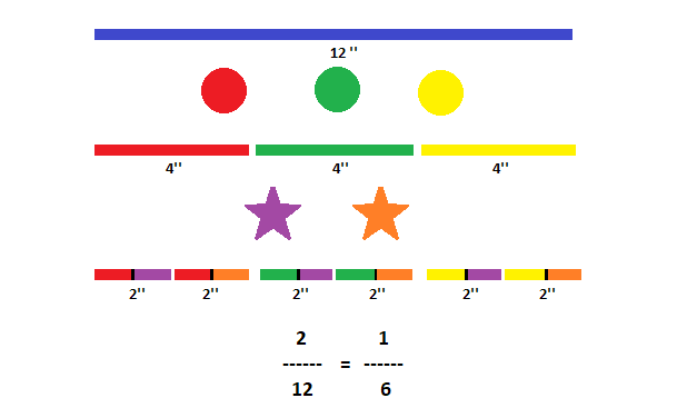
is a product of P(A) = and P(B)=. It gives us an intuition of why we took a product of the two probabilities. It will also be helpful to consider the bar as the probability space.
As a side note:
Suppose that A means that it rains today and B means that it rains tomorrow. If I know that it rained today, it is more likely that it will rain tomorrow, so p(B|A) > p(B).
In general, the probability of a conjunction is p(A and B) =p(A)p(B|A).
A constrained/conditional probability space is given by
p(A) =, where p(S)=1 and S is Sample space. Similarly, p(A|B) =
But what about when two events are dependent on each other?
Here is another way to think of such a case, the Bayes theorem illustrated below gives us a way to update the probability of a hypothesis, H in light of some body of data, D. That is event H and Event D are dependent. This way of thinking about Bayes’s theorem is called the diachronic inter-pretation. “Diachronic” means that something is happening over time; in this case the probability of the hypotheses changes, over time, as we see new data. p(H|D) =
In this interpretation, each term has a name:
- p(H) is the probability of the hypothesis before we see the data, called the prior probability, or just prior.
- p(H|D) is what we want to compute, the probability of the hypothesis after we see the data, called the posterior.
- p(D|H) is the probability of the data under the hypothesis, called the likelihood.
- p(D) is the probability of the data under any hypothesis, called the normalizing constant.
What is normalizing constant really? It is all the times the sympton/data occurs, that is all the times p(D) occurs in the absence or in the presence of hypotheses In this case, the value
is the normalizing constant.It can be extended from countably many hypotheses to uncountably many by replacing the sum by an integral.
It normalizes by restricting the probability in space [0,1]
Suppose we test for a rare disease and test is 99% right. Does this mean we have a 99% chance of testing positive?
No, however, this is a perfect case for bayes theorem.
if p(H) is 0.01 i.e 0.1% of the people have disease
we know p(H|D)= 0.99
p(D)= True Positive + True Negative where,
Hence on plugging in values we get p(H|D) = 9%
but Bayes is not a test to be done once, suppose we repeated the test and again tested positive, our prior would now be 9% instead of 0.1%. So the new probability would be 91%
An important insight to note is that, the Bayes theorem is only as good as your priors. As Nate Silverman puts it in his book signal and noise, debates between 0% prior beliefs and 100% prior beliefs are irreconciable…much like how liberals and conservatives cannot agree. Now, we have a formula to prove it.
In our own lives we follow our own priors to self-fullfilling prophecies internalizing the bayesian beliefs, so we must take everything with a grain of salt, be nuetral be stoic. We often suffer more in imagination than in reality - Seneca