After graduating from Pune Institute of Computer Technology with a placement at a reputed software firm,I decided to pursue my inclination towards datascience.I completed an online course on datascience from Dataquest.io, and then took the internship at NCL where I worked as a project intern at National Chemical Laboratory (NCL) with Dr. Leelavati Narlikar.

This blog post is a snapshot of all the duties I carried out there.

I performed Modified-Kmeans clustering, given sample of AGCT sequences generated from dirichlet distribution. The algorithm was as follows,

• Arbitarily partition data into k clusters, calculate $\oint_{k}$ for all k where

$\oint_{k}=log \prod_{n}^{i=1}P(X_{i} | Z)$

where X_i is probability value at each position in every sequence given Z viz probability of w.r.t each cluster

• Repeat
  • (re)assign each object to the cluster to which it is most similar based on $\oint_{k}$ calculate w.r.t to each k . Assign to cluster m if the value the maximizes on $\oint_{k}$
• Recompute $\oint$ for all k Until no change

I inititally designed an the above algorithm in pandas, a grave mistake. I varied the values of the length of the sequences and number of sequences and plotted a number of graphs w.r.t time as the performance metric.The result was not promising. The newly designed algorithm took the same time as the current system in place.I found out not quite suprisingly that time taken to convergence was directly ∝ to length of sequences and number of clusters. This is pretty much obvious,since there was a loop to measure probability at each position in each sequence and another loop to check likelihood for each cluster. I think we are slowly beginining to understand why Pandas was such a bad idea and why NumPy was so good. But just to be clear here are some reasons why,

1. Repeated apply function calls make pandas heavy in computation time
2. Indexing operation of pandas,aligns series on their indexes on every function call
3. NumPy array are contiguous blocks of memory so there is almost no indexing
4. Vectorization in numPy,applies an operation to all elements in an array

Here is my Psuedocode:

d = 100 /*len of seq*/
k=3   /* num of clusters */
n=100     /* num of Sequences */
psuedo= 1  /* psuedocount */

MAP(0..1)[n][4d]<--- ACGT[n][d]

Data[n][4d]<---MAP(0..1)[n][4d]

counts[0..k-1][4d]+= psuedo

totalcounts[0..k-1]+= 0
label[n]<--- randomized from 0 to k-1 /* randomly assign labels */

for i to n:
	counts[label[i]]+=Data[i] /* initialize */

for i to k:
	totalcounts[i]+= sum(counts[i][0:4])

Phi[0..k-1][4d]<--- loglikelihood(counts[0..k-1][4d],totalcounts[0..k-1])

while True:
	likelihood[n][k]<----Phi[0..k-1][4d] * Data[n][4d]
        new_label[n]<---maximize(likelihood[n][k])
	flag =0
	for i to n
		if(label[i]!=new_label[i])
			flag=1
			updatecounts(counts,totalcounts,label,new_label,Data,i)
	label[n]=new_label[n]
	Phi[0..k-1][4d]<--- loglikelihood(counts[0..k-1][4d],totalcounts)
        if(flag==0)
		break

loglikelihood(counts,totalcounts): /* take log,to prevent overflowing */
	for i to k:
		total = totalcounts[i]
		for j to 4d
			Phi[i][j] = log10(counts[i][j]/total)
	return Phi

minimize(likelihood[n * k],label):
	for i to n
		new_label[i]=maximize_by_index(likelihood[n])
	return new_label


updatecounts(counts,totalcounts,label,new_label,Data,i):
	counts[label[i]] -= Data[i]
	counts[new_label[i]] += Data[i]
	totalcounts[label[i]] -= 1
	totalcounts[new_label[i]] += 1

A data of a certain sample size took 60 seconds with pandas-style implementation now took 20 microseconds. I performed many checks by adding noise linearly to check the algorithm for robustness, I varied alpha in the dirichlets distribution progressively and got good results even as the data got increasingly noisy. I also added noise in columns by varrying the set of important features to find a breaking point for the algorithm.The algorithm starts breaking when there are only 30% meaningful columns.

Let me explain better with the following examples:

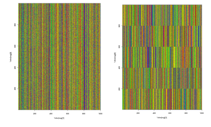
The colored lines visible above are noise added by me explictly they are color coded for A-C-G-T. the figure on the left is data generated that is randomized and the figure on the right is contains clusters generated after the algorithm was finished running.The plots are made using ggplot from R. I calculated the validity of the results by using the ARI(Adjusted Rand Index) from sklearn that compares the labels pre and post K-Means clustering. A perfect score is 1. I previously remarked on an algorithms breaking point,the metric I used to determine this point was the ARI.

Hope you liked this post. You may message on Disqus if you have any questions :)